Linear Regression from Scratch: GD, SGD and Scaling
Pure-Python linear regression: closed form, batch GD, mini-batch and SGD on seeded data. Real runs: divergence, and 140,538 epochs unscaled vs 2 scaled.
This is for developers who want to understand what "training" means before they hand it to a library: we fit a linear regression in plain Python, with no numpy, four ways. The closed form recovered the generator's slopes to within 0.01 in 0.47 ms; gradient descent reached the same loss in 2 epochs on scaled features, but needed 140,538 epochs on raw ones, and a learning rate just 6% too high sent the loss from 5,014 to 9.3 × 10¹² in 100 epochs. Every number below comes from one file you can copy and run.
This is lecture 1 of the series Machine learning from scratch (Python stdlib only). The later lectures build on the ideas here (a loss, a loop, a stopping rule): k-means clustering, a naive Bayes text classifier, from perceptron to neural network and a TF-IDF/BM25 search engine.
Environment: Python 3.9.6 standard library only (math, random, time, sys), Apple Silicon Mac (M1 Pro). The code uses no deprecated APIs, so it should run unchanged on Python 3.12+. All randomness is seeded.
The data: a generator whose answer we know
To check a learner you need data where the right answer is known. The generator below makes 600 listings with three features (floor area 20–150 m², building age 0–40 years, distance to the station 0.1–3.0 km) and a price:
price = 5.0 + 0.9 · area − 0.4 · age − 6.0 · km + Gaussian noise (σ = 4)
The rows are already in random order, so the first 480 are the training set and the last 120 the test set. With σ = 4 the noise alone has a variance of 16, so no model can get an MSE much below 16. That gives us a floor to judge against.
"""Linear regression from scratch: closed form vs gradient descent (Python stdlib only)."""
import math, random, sys, time

TRUE_B, TRUE_W = 5.0, [0.9, -0.4, -6.0]          # the answer we hope to recover

def make_data(n=600, seed=42):
    rng = random.Random(seed)
    X, y = [], []
    for _ in range(n):
        x = [rng.uniform(20, 150), rng.uniform(0, 40), rng.uniform(0.1, 3.0)]  # area, age, km
        X.append(x)
        y.append(TRUE_B + sum(w * v for w, v in zip(TRUE_W, x)) + rng.gauss(0, 4))
    return X, y

def add_bias(X):
    return [[1.0] + row for row in X]

def predict(row, w):
    return sum(a * b for a, b in zip(row, w))

def mse(A, y, w):
    return sum((predict(r, w) - t) ** 2 for r, t in zip(A, y)) / len(y)
add_bias puts a constant 1.0 in front of every row, so the intercept is just weight number 0 and every formula below handles it for free.
The closed form: one linear solve
Write the loss as L(w) = (1/n) · Σ (xᵢ·w − yᵢ)². Differentiate with respect to one weight wⱼ:
∂L/∂wⱼ = (2/n) · Σ (xᵢ·w − yᵢ) · xᵢⱼ
Stacked over all j, that is ∇L = (2/n) · Xᵀ(Xw − y). Keep this line in mind: it is the whole of gradient descent too. At the minimum the gradient is zero, which gives the normal equations XᵀX w = Xᵀy. With four weights, XᵀX is a 4 × 4 matrix, and we solve it with Gaussian elimination. Do not invert the matrix: solving is cheaper and more accurate.
# ---------- 1. closed form: solve (X^T X) w = X^T y ----------
def solve(M, v):
    """Gaussian elimination with partial pivoting."""
    d = len(v)
    M = [row[:] + [v[i]] for i, row in enumerate(M)]
    for c in range(d):
        p = max(range(c, d), key=lambda r: abs(M[r][c]))
        M[c], M[p] = M[p], M[c]
        for r in range(c + 1, d):
            f = M[r][c] / M[c][c]
            for k in range(c, d + 1):
                M[r][k] -= f * M[c][k]
    w = [0.0] * d
    for r in range(d - 1, -1, -1):
        w[r] = (M[r][d] - sum(M[r][k] * w[k] for k in range(r + 1, d))) / M[r][r]
    return w

def closed_form(A, y):
    d = len(A[0])
    XtX = [[sum(r[i] * r[j] for r in A) for j in range(d)] for i in range(d)]
    Xty = [sum(r[i] * t for r, t in zip(A, y)) for i in range(d)]
    return solve(XtX, Xty)
Output (weights are [intercept, area, age, km]):
Python 3.9.6  train 480  test 120
true       [5.000, 0.900, -0.400, -6.000]
closed    [4.063, 0.909, -0.394, -6.005]  train 16.6759  test 14.6532
true w    train 16.8045  test 14.6847
target: train MSE <= 16.6926
The three slopes are within 0.01 of the truth. The intercept is off by almost 1, and that is not a bug. The intercept is the predicted price at area 0, age 0 and distance 0, and no listing has an area below 20 m². Extrapolating that far magnifies tiny slope errors. Judge a regression on its predictions, not on whether the intercept looks right. The training MSE of 16.68 sits right at the noise floor of 16. The test MSE is lower (14.65), and the true w line shows why: even the generator's own weights score 16.80 on the training rows and 14.68 on the test rows. Those 120 test rows simply drew less noise. Note also that the fitted weights beat the true ones on the training set (16.68 < 16.80): least squares fits a little of the noise. On the test set the order flips back almost to a tie (14.65 vs 14.68).
The target line sets the goal for every gradient descent run below: get the training MSE within 0.1% of the closed-form optimum.
Batch gradient descent, from the same derivative
Gradient descent takes the gradient we just derived and walks downhill instead of solving for zero:
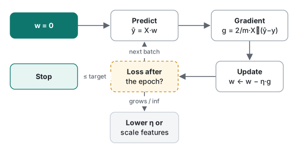
w ← w − η · (2/m) · Xᵀ(Xw − y)
η is the learning rate, and m is the number of rows used for one step. Using all n rows is batch GD; a random slice of 32 is mini-batch; one row at a time is stochastic GD (SGD). That makes it one function with a batch parameter:
# ---------- 2/3. batch, mini-batch and stochastic gradient descent ----------
def gd(A, y, lr, max_epochs, batch=None, target=None, seed=0, trace=None):
    rng = random.Random(seed)
    n, d = len(A), len(A[0])
    w, idx = [0.0] * d, list(range(n))
    bs = batch or n                                   # batch=None -> full batch
    for ep in range(1, max_epochs + 1):
        if batch:
            rng.shuffle(idx)
        for s in range(0, n, bs):
            rows = idx[s:s + bs]
            g = [0.0] * d
            for i in rows:
                e = predict(A[i], w) - y[i]           # residual
                for j in range(d):
                    g[j] += e * A[i][j]
            k = 2.0 / len(rows)                       # d/dw of mean squared error
            w = [wj - lr * k * gj for wj, gj in zip(w, g)]
        try:
            loss = mse(A, y, w)
        except OverflowError:
            loss = math.inf
        if trace is not None and ep in trace:
            print(f"  epoch {ep:>5}  loss {loss:.4g}")
        if not math.isfinite(loss):
            return w, ep, loss, "diverged"
        if target is not None and loss <= target:
            return w, ep, loss, "reached"
    return w, max_epochs, loss, "not reached"
The try/except OverflowError is there because of a real crash. In pure Python, a diverging run eventually stops with OverflowError: (34, 'Result too large') when it squares a float near 1e308, instead of quietly producing inf as numpy would. An epoch is one pass over the training rows, so batch GD makes 1 update per epoch, mini-batch 32 makes 15 and SGD makes 480.
What goes wrong 1: a learning rate that is too high
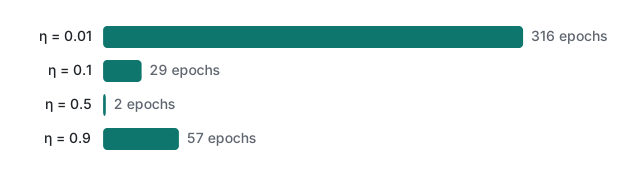
We ran full-batch GD on standardized features (next section) with six learning rates:
[learning-rate sweep, scaled features, full batch]
lr 0.01  reached   epoch   316  loss 16.69
lr 0.1   reached   epoch    29  loss 16.69
lr 0.5   reached   epoch     2  loss 16.69
lr 0.9   reached   epoch    57  loss 16.69
lr 1.0   diverged  epoch  2917  loss inf
lr 1.1   diverged  epoch  1193  loss inf
Two things stand out. Bigger is not faster: 0.5 needs 2 epochs, but 0.9 needs 57. And between 0.9 and 1.0 there is a cliff. Here is the loss of the diverging runs, printed by the trace argument:
[lr 1.1]
  epoch     1  loss 7219
  epoch     2  loss 1.037e+04
  epoch     3  loss 1.507e+04
  epoch     5  loss 3.29e+04
  epoch    10  loss 2.858e+05
  epoch    20  loss 5.169e+07
  epoch    30  loss 1.616e+10
[lr 1.0]
  epoch     1  loss 5014
  epoch    10  loss 8174
  epoch   100  loss 9.325e+12
  epoch   500  loss 3.354e+54
  epoch  1000  loss 2.954e+106
  epoch  2000  loss 2.292e+210
  epoch  2500  loss 2.019e+262
Note what the table above hid. It said lr 1.0 "diverged at epoch 2917", but the loss was already 9.3e12 at epoch 100. A check for inf or NaN fires thousands of epochs late. In real training code, also stop when the loss exceeds the loss of the first epoch. That check would have stopped both runs within 10 epochs.
Where is the cliff? For MSE the loss is a bowl whose curvature is the Hessian H = (2/n)XᵀX. Along the direction of its largest eigenvalue λmax, each step multiplies the error by (1 − η·λmax). If that factor is below −1 the error flips sign and grows: GD diverges when η > 2/λmax. We computed λ with power iteration:
# ---------- why a learning rate is "too high" ----------
def curvature(A):
    """largest / smallest eigenvalue of the MSE Hessian (2/n) X^T X (power iteration)"""
    n, d = len(A), len(A[0])
    H = [[2 / n * sum(r[i] * r[j] for r in A) for j in range(d)] for i in range(d)]
    out = []
    for step in (lambda v: [predict(row, v) for row in H], lambda v: solve(H, v)):
        v = [1.0] * d
        for _ in range(300):
            u = step(v)
            nrm = math.sqrt(sum(x * x for x in u))
            v = [x / nrm for x in u]
        out.append(predict(v, [predict(row, v) for row in H]))
    return out                                        # [lambda_max, lambda_min]
unscaled  lambda_max 1.745e+04  lambda_min 0.1563  condition 111,625.8  max stable lr 2/lambda_max = 0.0001146
scaled    lambda_max 2.127  lambda_min 1.878  condition 1.1  max stable lr 2/lambda_max = 0.9403
The theory matches the runs exactly: 0.9 < 0.9403 converged, and 1.0 > 0.9403 diverged. It also explains why 0.9 was slow. With 1 − 0.9 × 2.127 = −0.91, the weights overshoot back and forth across the valley and shrink the error by only 9% per epoch. The best fixed rate is 2/(λmax + λmin) = 0.499, which is why 0.5 needed just 2 epochs.
What goes wrong 2: features on different scales
The unscaled line above is the second failure. Area runs up to 150, while the bias column is always 1, so the bowl is 111,626 times steeper in one direction than in another. The learning rate must be small enough for the steep direction (below 0.000115), and at that rate the shallow direction barely moves. Just past the limit, at 1.2e-4, raw features diverge as well:
[unscaled, lr 1.2e-4]
  epoch     1  loss 6047
  epoch     2  loss 7201
  epoch     3  loss 8584
  epoch     5  loss 1.222e+04
  epoch    10  loss 2.972e+04
  epoch    50  loss 3.782e+07
  epoch   100  loss 2.883e+11
  epoch   200  loss 1.676e+19
  epoch   400  loss 5.661e+34
The fix is to standardize each feature to mean 0 and standard deviation 1. Compute the mean and standard deviation on the training rows only and reuse them for the test rows. Computing them on all 600 rows lets test information leak into training. After training, convert the weights back so they are in the original units:
# ---------- 4. feature scaling (standardize with TRAIN statistics only) ----------
def fit_scaler(X):
    cols = list(zip(*X))
    mean = [sum(c) / len(c) for c in cols]
    std = [math.sqrt(sum((v - m) ** 2 for v in c) / len(c)) for c, m in zip(cols, mean)]
    return mean, std

def scale(X, mean, std):
    return [[(v - m) / s for v, m, s in zip(r, mean, std)] for r in X]

def unscale(w, mean, std):
    """weights learned on scaled features -> weights in original units"""
    ws = [wj / s for wj, s in zip(w[1:], std)]
    return [w[0] - sum(wj * m for wj, m in zip(ws, mean))] + ws
Epochs to the same target, with and without scaling (raw features at 1.1e-4, just under their stability limit):
[epochs to target: scaled vs unscaled, full batch]
scaled   lr 0.5     reached at epoch 2  [4.312, 0.906, -0.394, -5.980]
scaled   lr 0.9     reached at epoch 57
  epoch  1000  loss 34.73
  epoch 10000  loss 18.55
  epoch 20000  loss 17.73
  epoch 100000  loss 16.74
unscaled lr 1.1e-4  reached at epoch 140538  loss 16.6926  100.7 s  [3.610, 0.911, -0.389, -5.913]

That is 2 epochs against 140,538, from one preprocessing step. The unscaled run also shows a trap. Without --long the script stops at epoch 20,000, where the loss of 17.73 is only 6% above the optimum and looks nearly converged. Its weights tell a different story:
unscaled lr 1.1e-4 not reached at epoch 20000 loss 17.7341 14.1 s [0.483, 0.925, -0.357, -5.196]
The km weight is −5.20 instead of −6.0, and the intercept is 0.48 instead of about 4. Even at the 0.1% target, after 140,538 epochs, the km weight was still −5.913 against −6.005 from the closed form. A loss that has nearly stopped falling can still hide a lot of error in the weights along the shallow direction. If you stop when the loss stops moving much, you may stop with the wrong model.
Mini-batch and stochastic gradient descent
Same function, batch=32 and batch=1, scaled features, shuffle seed 1, a few learning rates each:
[mini-batch and SGD, scaled, shuffle seed 1]
batch 32  lr 0.02   reached     epoch   11  loss 16.6874  test 14.7088  [4.066, 0.908, -0.395, -5.974]
batch 32  lr 0.05   reached     epoch    4  loss 16.6845  test 14.6414  [4.045, 0.908, -0.388, -6.005]
batch 32  lr 0.1    reached     epoch    9  loss 16.6906  test 14.7560  [3.942, 0.910, -0.399, -5.992]
batch 32  lr 0.2    reached     epoch  290  loss 16.6893  test 14.6619  [4.195, 0.907, -0.390, -6.058]
batch 1   lr 0.001  reached     epoch    7  loss 16.6910  test 14.7085  [4.080, 0.908, -0.392, -6.007]
batch 1   lr 0.002  reached     epoch    4  loss 16.6845  test 14.6064  [4.116, 0.910, -0.391, -6.045]
batch 1   lr 0.005  reached     epoch  184  loss 16.6837  test 14.6878  [4.111, 0.909, -0.392, -6.053]
batch 1   lr 0.01   reached     epoch    3  loss 16.6805  test 14.6572  [3.868, 0.910, -0.389, -5.972]
batch 1   lr 0.02   not reached epoch 2000  loss 17.7942  test 15.5188  [7.181, 0.882, -0.411, -6.256]
batch 1   lr 0.05   not reached epoch 2000  loss 17.8677  test 15.5023  [7.453, 0.885, -0.399, -6.600]
[SGD lr 0.005, shuffle seeds 1-5]
  epochs: [184, 15, 17, 163, 68]
This output did not match what we expected, and it is the most useful result in this section.
- The epoch counts are not monotonic in the learning rate. For SGD, 0.002 took 4 epochs, 0.005 took 184 and 0.01 took 3. A single-row gradient is a noisy estimate of the full one, so the weights never settle at the optimum. They jitter around it, and "reached the target" means one jitter happened to land inside the 0.1% band. The same rate of 0.005 took 184, 15, 17, 163 and 68 epochs depending only on the shuffle seed. Never compare SGD settings on one seed.
- A too-high rate does not explode, it plateaus. At 0.02 and 0.05, SGD stayed finite but stuck near a loss of 17.8, and the intercept drifted to 7.2–7.5. The jitter is bigger than the target band, so it never lands inside it. That failure is quieter than divergence and easier to miss.
- Mini-batches average the noise away. At 32 rows per step (15 updates per epoch), every rate from 0.02 to 0.1 reached the target in 4 to 11 epochs. At 0.2 the jitter grew, and it took 290.
On 480 rows, SGD buys nothing over batch GD. Its strengths show elsewhere: it never needs the whole dataset in memory, and it can keep learning as new rows arrive. In practice SGD is run with a learning rate that decays over time, so the jitter shrinks as training goes on. Our loop keeps the rate fixed so the effect is visible.
Wall time and the test set
Best of 5 runs each, from start until the target loss. The SGD row uses rate 0.005 with seed 1, the unlucky 184-epoch case:
[wall time, best of 5]
closed form               0.47 ms
batch GD lr 0.5           1.39 ms
batch GD lr 0.9          39.69 ms
mini-batch 32             3.28 ms
SGD (batch 1)           212.59 ms

test MSE  closed 14.6532  batch GD 14.6333
The GD timings include computing the full training loss after every epoch, which is how we know when to stop. On this problem the closed form wins outright: one pass to build a 4 × 4 matrix and one tiny solve. The two test MSEs differ by 0.02, well inside the noise. Stopping 0.1% short of the training optimum did no harm, and was even slightly better on this particular test set.
| Closed form | GD (batch / mini-batch) | SGD | |
|---|---|---|---|
| Cost | Builds XᵀX: O(n·d²), then solves it: O(d³) | O(n·d) per epoch × number of epochs | O(d) per update |
| Use it when | d up to a few thousand and the data fits in memory | d is large (d³ is too much) or you add a penalty with no closed form, such as L1 | data streams in, does not fit in memory, or the model must keep updating online |
| Needs scaling | No | Yes (2 vs 140,538 epochs here) | Yes |
| Hyperparameters | None | Learning rate, stopping rule | Learning rate (and its decay), batch size, seed |
| Fails when | XᵀX is singular, for example a duplicated feature. Use ridge or a least-squares solver | η > 2/λmax; slow if poorly conditioned | Rate too high: loss keeps bouncing above the target |
Honest limits
- It is slow because it has no numpy. Every multiply is an interpreted Python operation. 480 rows × 4 weights is fine; a million rows with a hundred features is not. The 140,538-epoch unscaled run took 100.7 seconds for a problem the closed form solves in under a millisecond. A vectorized library would make each epoch far cheaper.
- The normal equations are not how libraries solve it. Forming XᵀX squares the conditioning of the problem. In float64 that is harmless at a condition number of about 10⁵, but it loses digits on nearly collinear features. What scikit-learn would use instead:
LinearRegression(a least-squares solver based on matrix decomposition, without forming XᵀX),StandardScalerfor the scaling step andSGDRegressorfor the SGD variant. We name them here and did not run them, because the point of this series is to see the mechanism. - One synthetic dataset. The features are independent and uniform, and the noise is Gaussian, so the problem is very clean. Correlated features push the condition number up even after scaling. Outliers punish squared error, and a model that should not be linear cannot be fixed by any of the methods above.
- Small, fixed-rate sweeps. We tried a handful of learning rates and one or five seeds, not a systematic search, and used no learning-rate decay. Real training code adds a schedule and stops early when the loss rises.
Run it yourself
The blocks above, from top to bottom, form linreg.py. Add this driver at the end. python3 linreg.py ran in 27 seconds here; python3 linreg.py --long also lets the unscaled run reach the target, which adds about 100 seconds.
def fmt(w):
    return "[" + ", ".join(f"{v:.3f}" for v in w) + "]"

def best_of(fn, k=5):
    ts = []
    for _ in range(k):
        t = time.perf_counter(); fn(); ts.append(time.perf_counter() - t)
    return min(ts)

if __name__ == "__main__":
    LONG = "--long" in sys.argv                       # unscaled run until it converges (minutes)
    X, y = make_data()
    cut = int(len(X) * 0.8)                           # rows are already random: 480 / 120
    Xtr, ytr, Xte, yte = X[:cut], y[:cut], X[cut:], y[cut:]
    Atr, Ate = add_bias(Xtr), add_bias(Xte)
    print(f"Python {sys.version.split()[0]}  train {len(Xtr)}  test {len(Xte)}")
    print("true      ", fmt([TRUE_B] + TRUE_W))

    w_cf = closed_form(Atr, ytr)
    best = mse(Atr, ytr, w_cf)
    print(f"closed    {fmt(w_cf)}  train {best:.4f}  test {mse(Ate, yte, w_cf):.4f}")
    w_true = [TRUE_B] + TRUE_W                        # noise only: the floor for any model
    print(f"true w    train {mse(Atr, ytr, w_true):.4f}  test {mse(Ate, yte, w_true):.4f}")
    target = best * 1.001                             # within 0.1% of the optimum
    print(f"target: train MSE <= {target:.4f}")

    mean, std = fit_scaler(Xtr)
    Str, Ste = add_bias(scale(Xtr, mean, std)), add_bias(scale(Xte, mean, std))
    for name, A in (("unscaled", Atr), ("scaled", Str)):
        hi, lo = curvature(A)
        print(f"{name:<9} lambda_max {hi:.4g}  lambda_min {lo:.4g}  "
              f"condition {hi/lo:,.1f}  max stable lr 2/lambda_max = {2/hi:.4g}")

    print("\n[learning-rate sweep, scaled features, full batch]")
    for lr in (0.01, 0.1, 0.5, 0.9, 1.0, 1.1):
        w, ep, loss, st = gd(Str, ytr, lr, 5000, target=target)
        print(f"lr {lr:<5} {st:<9} epoch {ep:>5}  loss {loss:.4g}")
    print("[lr 1.1]")
    gd(Str, ytr, 1.1, 30, trace={1, 2, 3, 5, 10, 20, 30})
    print("[lr 1.0]")
    gd(Str, ytr, 1.0, 5000, trace={1, 10, 100, 500, 1000, 2000, 2500})
    print("[unscaled, lr 1.2e-4]")
    gd(Atr, ytr, 1.2e-4, 400, trace={1, 2, 3, 5, 10, 50, 100, 200, 400})

    print("\n[epochs to target: scaled vs unscaled, full batch]")
    w_s, ep, loss, st = gd(Str, ytr, 0.5, 5000, target=target)
    print(f"scaled   lr 0.5     {st} at epoch {ep}  {fmt(unscale(w_s, mean, std))}")
    w_s9, ep, loss, st = gd(Str, ytr, 0.9, 5000, target=target)
    print(f"scaled   lr 0.9     {st} at epoch {ep}")
    t = time.perf_counter()
    w_u, ep, loss, st = gd(Atr, ytr, 1.1e-4, 600000 if LONG else 20000, target=target,
                           trace={1000, 10000, 20000, 100000, 200000, 300000})
    print(f"unscaled lr 1.1e-4  {st} at epoch {ep}  loss {loss:.4f}  "
          f"{time.perf_counter()-t:.1f} s  {fmt(w_u)}")

    print("\n[mini-batch and SGD, scaled, shuffle seed 1]")
    for bs, lrs in ((32, (0.02, 0.05, 0.1, 0.2)), (1, (0.001, 0.002, 0.005, 0.01, 0.02, 0.05))):
        for lr in lrs:
            w, ep, loss, st = gd(Str, ytr, lr, 2000, batch=bs, target=target, seed=1)
            print(f"batch {bs:<3} lr {lr:<6} {st:<11} epoch {ep:>4}  loss {loss:.4f}  "
                  f"test {mse(Ste, yte, w):.4f}  {fmt(unscale(w, mean, std))}")
    print("[SGD lr 0.005, shuffle seeds 1-5]")
    print("  epochs:", [gd(Str, ytr, 0.005, 2000, batch=1, target=target, seed=sd)[1]
                       for sd in range(1, 6)])

    print("\n[wall time, best of 5]")
    print(f"closed form           {best_of(lambda: closed_form(Atr, ytr))*1000:8.2f} ms")
    for lbl, lr, kw in (("batch GD lr 0.5", 0.5, {}), ("batch GD lr 0.9", 0.9, {}),
                        ("mini-batch 32", 0.05, {"batch": 32, "seed": 1}),
                        ("SGD (batch 1)", 0.005, {"batch": 1, "seed": 1})):
        ms = best_of(lambda: gd(Str, ytr, lr, 5000, target=target, **kw)) * 1000
        print(f"{lbl:<21} {ms:8.2f} ms")

    print(f"\ntest MSE  closed {mse(Ate, yte, w_cf):.4f}  batch GD {mse(Ste, yte, w_s):.4f}")
The losses, epochs and weights are deterministic for a given seed. Wall times will differ on your machine, but their ratios should not.
Next in the series: k-means clustering from scratch, where the loop is "assign, then update" instead of "gradient, then step". For another hands-on timing comparison in this style, see sorting algorithms measured in C.
FAQ
Why does gradient descent blow up when the learning rate is too high?
For mean squared error the loss is a bowl whose steepest curvature is the largest eigenvalue λmax of (2/n)XᵀX. Any learning rate above 2/λmax overshoots further on every step. On our standardized data 2/λmax was 0.94: a rate of 0.9 converged, 1.0 went from a loss of 5,014 to 9.3e12 in 100 epochs.
How much does feature scaling actually speed up gradient descent?
On the same 480 rows, standardized features reached the target loss in 2 epochs (learning rate 0.5). Raw features needed 140,538 epochs at the largest stable learning rate, because the curvature differed by a factor of 111,626 between directions.
Should I use the closed form or gradient descent for linear regression?
With a few features and data that fits in memory, use the closed form (a least-squares solver): it took 0.47 ms here versus 1.39 ms for the best-tuned gradient descent. Use gradient descent or SGD when there are very many features, the data streams in, or you add a penalty with no closed form.