Perceptron to Neural Network in Pure Python, Measured
The perceptron learns AND and OR but never XOR. A hand-written backprop net solves it, yet often gets stuck: 100 seeds, a gradient check, two moons.
If you have read that "a perceptron cannot learn XOR" and that "backpropagation fixes it", this article shows both claims as real program output, in about 150 lines of Python you can run without installing anything. The perceptron solves AND in 6 epochs and OR in 4, and on XOR it cycles through the same four weight vectors forever. A 2-H-1 network with hand-written backprop solves XOR, but only 41 of 100 random starts succeed with 2 hidden units. The surprise was why the other 59 failed.
This is lecture 4 of the series Machine learning from scratch (Python stdlib only). Lecture 1 was linear regression with gradient descent, lecture 2 k-means clustering, lecture 3 a naive Bayes text classifier. The last lecture is a TF-IDF and BM25 search engine.
Environment: Python 3.9.6 standard library only (math, random, time), Apple Silicon Mac (M1 Pro). Every seed is fixed, so you should get the same numbers.
The perceptron rule on AND, OR and XOR
The perceptron outputs 1 if w1·x1 + w2·x2 + b > 0, else 0. The learning rule changes the weights only when the answer is wrong: add the input when the answer should have been 1, subtract it when it should have been 0. The perceptron convergence theorem says this stops after a finite number of mistakes if a separating line exists.
# perceptron.py - Rosenblatt perceptron rule on AND / OR / XOR (stdlib only)
DATA = [(0, 0), (0, 1), (1, 0), (1, 1)]
TARGETS = {"AND": [0, 0, 0, 1], "OR": [0, 1, 1, 1], "XOR": [0, 1, 1, 0]}

def train(targets, lr=1.0, max_epochs=100):
    w1 = w2 = b = 0.0
    history = []
    for epoch in range(1, max_epochs + 1):
        errors = 0
        for (x1, x2), t in zip(DATA, targets):
            y = 1 if w1 * x1 + w2 * x2 + b > 0 else 0
            if y != t:                       # update only on a mistake
                w1 += lr * (t - y) * x1
                w2 += lr * (t - y) * x2
                b += lr * (t - y)
                errors += 1
        history.append((epoch, errors, (w1, w2, b)))
        if errors == 0:
            return epoch, (w1, w2, b), history
    return None, (w1, w2, b), history

for name, t in TARGETS.items():
    epoch, w, hist = train(t)
    if epoch:
        print(f"{name}: converged after {epoch} epochs, w1={w[0]} w2={w[1]} b={w[2]}")
    else:
        print(f"{name}: NOT converged in {len(hist)} epochs")
        for e, err, ww in hist[:6] + hist[-2:]:
            print(f"  epoch {e:3d} errors={err} w={ww}")
        seen = {}
        for e, err, ww in hist:
            if ww in seen:
                print(f"  weights at epoch {e} repeat epoch {seen[ww]} -> cycle of {e - seen[ww]}")
                break
            seen[ww] = e
AND: converged after 6 epochs, w1=2.0 w2=1.0 b=-2.0
OR: converged after 4 epochs, w1=1.0 w2=1.0 b=0.0
XOR: NOT converged in 100 epochs
  epoch   1 errors=2 w=(-1.0, 0.0, 0.0)
  epoch   2 errors=3 w=(-1.0, 0.0, 1.0)
  epoch   3 errors=4 w=(-1.0, 0.0, 1.0)
  epoch   4 errors=4 w=(-1.0, 0.0, 1.0)
  …
  epoch 100 errors=4 w=(-1.0, 0.0, 1.0)
  weights at epoch 3 repeat epoch 2 -> cycle of 1
The AND line 2·x1 + 1·x2 − 2 > 0 is true only for (1, 1). Note the asymmetric weights: the rule stops at the first line that works, not the nicest one.
XOR is the interesting output. From epoch 3 on, every one of the four samples is wrong in every epoch, yet the weights at the end of each epoch are identical. Tracing one epoch by hand shows why. Starting from (−1, 0, 1): (0,0) fires wrongly, so b drops to 0; (0,1) does not fire, so w2 and b rise to (−1, 1, 1); (1,0) does not fire, so we reach (0, 1, 2); (1,1) fires wrongly and subtracts (1, 1, 1), giving back (−1, 0, 1). Each fix undoes the previous one. No single line puts (0,1) and (1,0) on one side and (0,0) and (1,1) on the other, so the convergence theorem gives no guarantee and the rule loops forever. A "max epochs" limit is not optional.
A 2-H-1 network with backprop written by hand
The fix is a hidden layer: 2 inputs, H hidden units with tanh, 1 sigmoid output, binary cross-entropy loss. With a sigmoid output and cross-entropy, the error at the output's pre-activation is simply y − t. The hidden error multiplies that by the outgoing weight and by the derivative of tanh, which is 1 − h² when written in terms of the output h.
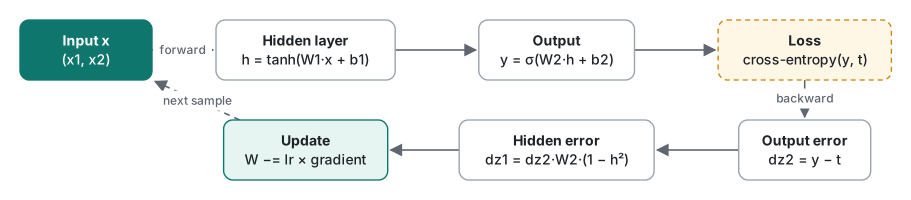
This file is the core of the article. The later scripts import Net from it, so save it as xor_mlp.py.
# xor_mlp.py - 2-H-1 network, backprop by hand, trained on XOR (stdlib only)
# usage: python3 xor_mlp.py [tanh|sigmoid] [init_scale] [seeds]
import math, random, sys, time

X = [(0.0, 0.0), (0.0, 1.0), (1.0, 0.0), (1.0, 1.0)]
T = [0.0, 1.0, 1.0, 0.0]

def sigmoid(z):
    return 1.0 / (1.0 + math.exp(-z))

ACTS = {  # activation, and its derivative written in terms of the output h
    "tanh":    (math.tanh, lambda h: 1.0 - h * h),
    "sigmoid": (sigmoid,   lambda h: h * (1.0 - h)),
}

class Net:
    def __init__(self, n_in, n_hid, rng, act="tanh", scale=1.0):
        self.f, self.df = ACTS[act]
        self.W1 = [[rng.uniform(-scale, scale) for _ in range(n_in)] for _ in range(n_hid)]
        self.b1 = [0.0] * n_hid
        self.W2 = [rng.uniform(-scale, scale) for _ in range(n_hid)]
        self.b2 = 0.0

    def forward(self, x):
        h = [self.f(sum(w * xi for w, xi in zip(row, x)) + b)
             for row, b in zip(self.W1, self.b1)]
        y = sigmoid(sum(w * hj for w, hj in zip(self.W2, h)) + self.b2)
        return h, y

    def loss(self, x, t):                         # binary cross-entropy
        y = min(max(self.forward(x)[1], 1e-12), 1 - 1e-12)
        return -(t * math.log(y) + (1 - t) * math.log(1 - y))

    def backward(self, x, t):
        h, y = self.forward(x)
        dz2 = y - t                               # dL/dz2 for sigmoid + BCE
        gW2 = [dz2 * hj for hj in h]
        dz1 = [dz2 * w * self.df(hj) for w, hj in zip(self.W2, h)]
        gW1 = [[d * xi for xi in x] for d in dz1]
        return gW1, dz1, gW2, dz2                 # dz1 = gb1, dz2 = gb2

    def step(self, grads, lr):
        gW1, gb1, gW2, gb2 = grads
        for j in range(len(self.W2)):
            for i in range(len(self.W1[j])):
                self.W1[j][i] -= lr * gW1[j][i]
            self.b1[j] -= lr * gb1[j]
            self.W2[j] -= lr * gW2[j]
        self.b2 -= lr * gb2

def train_xor(n_hid, seed, act="tanh", scale=1.0, lr=0.5, max_epochs=5000):
    rng = random.Random(seed)
    net = Net(2, n_hid, rng, act, scale)
    order = list(range(4))
    for epoch in range(1, max_epochs + 1):
        rng.shuffle(order)
        for k in order:                           # plain SGD, one sample at a time
            net.step(net.backward(X[k], T[k]), lr)
        if all(abs(net.forward(x)[1] - t) < 0.1 for x, t in zip(X, T)):
            return epoch, net
    return None, net

if __name__ == "__main__":
    act = sys.argv[1] if len(sys.argv) > 1 else "tanh"
    scale = float(sys.argv[2]) if len(sys.argv) > 2 else 1.0
    seeds = range(int(sys.argv[3]) if len(sys.argv) > 3 else 100)
    for n_hid in (2, 4, 8):
        t0 = time.perf_counter()
        solved = sorted(e for e in (train_xor(n_hid, s, act, scale)[0] for s in seeds) if e)
        dt = time.perf_counter() - t0
        med = solved[len(solved) // 2] if solved else "-"
        rng_ = f"{solved[0]}-{solved[-1]}" if solved else "-"
        print(f"{act} init±{scale} hidden={n_hid}: solved {len(solved)}/{len(seeds)}  "
              f"median epochs {med}  range {rng_}  time {dt:.1f}s")
"Solved" means all four outputs are within 0.1 of their targets. A run that has not solved XOR after 5,000 epochs counts as stuck.
100 seeds per setting: how often it gets stuck
The first version of this code drew initial weights from ±0.71 (1/√2, a common fan-in rule). It solved XOR in only 13, 21 and 48 of 100 seeds for 2, 4 and 8 hidden units. That was far worse than expected, so we varied the initial range and also tried a sigmoid hidden layer:
$ python3 xor_mlp.py tanh 1.0
tanh init±1.0 hidden=2: solved 41/100  median epochs 68  range 33-101  time 7.1s
tanh init±1.0 hidden=4: solved 73/100  median epochs 54  range 30-96  time 5.3s
tanh init±1.0 hidden=8: solved 97/100  median epochs 37  range 23-81  time 1.2s
$ python3 xor_mlp.py tanh 0.5
tanh init±0.5 hidden=2: solved 0/100  median epochs -  range -  time 13.1s
tanh init±0.5 hidden=4: solved 1/100  median epochs 81  range 81-81  time 18.4s
tanh init±0.5 hidden=8: solved 5/100  median epochs 89  range 77-93  time 29.7s
$ python3 xor_mlp.py tanh 2.0
tanh init±2.0 hidden=2: solved 54/100  median epochs 47  range 22-115  time 6.1s
tanh init±2.0 hidden=4: solved 97/100  median epochs 30  range 15-235  time 0.8s
tanh init±2.0 hidden=8: solved 100/100  median epochs 17  range 9-40  time 0.1s
$ python3 xor_mlp.py sigmoid 1.0
sigmoid init±1.0 hidden=2: solved 63/100  median epochs 392  range 170-3482  time 5.9s
sigmoid init±1.0 hidden=4: solved 100/100  median epochs 327  range 173-1046  time 1.4s
sigmoid init±1.0 hidden=8: solved 100/100  median epochs 230  range 143-443  time 1.6s
$ python3 xor_mlp.py sigmoid 0.5
sigmoid init±0.5 hidden=2: solved 77/100  median epochs 488  range 330-3128  time 4.2s
sigmoid init±0.5 hidden=4: solved 100/100  median epochs 446  range 326-849  time 1.8s
sigmoid init±0.5 hidden=8: solved 100/100  median epochs 383  range 298-507  time 2.6s
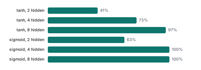
Three things stand out:
- More hidden units help a lot. With tanh at ±1.0, success goes 41 → 73 → 97 out of 100, and the median epochs to solve drop 68 → 54 → 37.
- Runs that succeed do so quickly. No tanh run at ±1.0 took more than 101 epochs. Rerunning with a 2,000-epoch limit gave exactly the same 41, 73 and 97, so the extra 3,000 epochs rescued no stuck run. If a tanh run has not solved XOR within a few hundred epochs, more patience will not help.
- The initial range matters as much as the architecture. At ±0.5, tanh almost never succeeds (0, 1, 5 of 100). A sigmoid hidden layer at the same ±0.5 solved 77, 100 and 100. It is slower (median 488 epochs for H=2) but much harder to break.
The time column is mostly the stuck runs: each one runs the full 5,000 epochs. That is why 100 seeds of the 8-unit net at ±0.5 took 29.7 s while the 8-unit net at ±2.0 took 0.1 s.
What a stuck run looks like
"Stuck in a local minimum" is the usual explanation. We counted instead:
# failmodes.py - what do the stuck runs look like?
import sys
from collections import Counter
from xor_mlp import train_xor, X

act, scale, n_hid = sys.argv[1], float(sys.argv[2]), int(sys.argv[3])
kinds, example = Counter(), {}
for seed in range(100):
    epoch, net = train_xor(n_hid, seed, act, scale)
    if epoch:
        continue
    biggest = max(abs(w) for row in net.W1 for w in row)
    outs = tuple(round(net.forward(x)[1], 2) for x in X)
    kind = "collapsed (weights ~0)" if biggest < 1e-6 else "local minimum"
    kinds[kind] += 1
    example.setdefault(kind, (seed, outs, f"{biggest:.1e}"))
print(dict(kinds))
for k, v in example.items():
    print(f"  {k}: seed {v[0]} outputs {v[1]} max|W1| {v[2]}")
$ python3 failmodes.py tanh 1.0 2
{'collapsed (weights ~0)': 54, 'local minimum': 5}
  collapsed (weights ~0): seed 0 outputs (0.49, 0.49, 0.49, 0.49) max|W1| 6.2e-49
  local minimum: seed 23 outputs (0.0, 1.0, 0.41, 0.41) max|W1| 6.4e+00
$ python3 failmodes.py tanh 1.0 4
{'collapsed (weights ~0)': 27}
  collapsed (weights ~0): seed 0 outputs (0.47, 0.47, 0.47, 0.47) max|W1| 5.1e-49
$ python3 failmodes.py sigmoid 1.0 2
{'local minimum': 37}
  local minimum: seed 8 outputs (0.0, 1.0, 0.51, 0.51) max|W1| 1.1e+01
$ python3 failmodes.py sigmoid 0.5 2
{'local minimum': 23}
  local minimum: seed 12 outputs (0.0, 0.67, 0.67, 0.67) max|W1| 9.7e+00
For tanh, 54 of the 59 failures with 2 hidden units, and all 27 with 4, were not local minima at all. Every hidden weight had shrunk to around 1e-49 and the network answered about 0.5 for every input. Our reading of why: when all weights are zero, tanh outputs 0, so the output weights get no gradient, and with zero output weights the hidden weights get none either. That point is stationary. Near it, tanh is almost linear, so the whole network behaves like a linear model, and the best linear model for XOR is "always 0.5". Gradient descent then pulls the weights toward zero. Small initial weights start the run inside that pull, which is why ±0.5 failed almost every time.
The sigmoid hidden layer never collapsed in our runs. Its failures were genuine local minima: one or two inputs learned perfectly, and the rest shared a single in-between answer (0.51 and 0.67 in the examples above). Those are the textbook case, and more hidden units removed them (100/100 at H=4).
Gradient checking: is the backward pass right?
A wrong derivative does not crash. It trains slowly, or a bit worse, and you blame the learning rate. The check is cheap: nudge each parameter by ±eps, measure the loss change, and compare with what backward returned.
# gradcheck.py - compare backprop gradients with central differences
import random
from xor_mlp import Net, X, T

def flat(net):
    return [w for row in net.W1 for w in row] + net.b1 + net.W2 + [net.b2]

def load(net, v):
    k, n_in, n_hid = 0, len(net.W1[0]), len(net.W2)
    for row in net.W1:
        row[:] = v[k:k + n_in]; k += n_in
    net.b1 = v[k:k + n_hid]; k += n_hid
    net.W2 = v[k:k + n_hid]; k += n_hid
    net.b2 = v[k]

def flat_grads(g):
    gW1, gb1, gW2, gb2 = g
    return [w for row in gW1 for w in row] + gb1 + gW2 + [gb2]

def check(net, eps, broken=False):
    if broken:                                  # simulate a classic bug: forget tanh'
        net.df = lambda h: 1.0
    worst_abs = worst_rel = 0.0
    for x, t in zip(X, T):
        p = flat(net)
        ana = flat_grads(net.backward(x, t))
        for k in range(len(p)):
            q = p[:]; q[k] += eps; load(net, q); lp = net.loss(x, t)
            q[k] -= 2 * eps;      load(net, q); lm = net.loss(x, t)
            load(net, p)
            num = (lp - lm) / (2 * eps)
            d = abs(num - ana[k])
            worst_abs = max(worst_abs, d)
            worst_rel = max(worst_rel, d / max(abs(num) + abs(ana[k]), 1e-12))
    return worst_abs, worst_rel, len(p)

for act in ("tanh", "sigmoid"):
    for eps in (1e-2, 1e-4, 1e-6, 1e-8):
        a, r, n = check(Net(2, 4, random.Random(42), act), eps)
        print(f"{act:7s} eps={eps:.0e}  max abs diff {a:.2e}  max rel diff {r:.2e}  ({n} params x 4 samples)")
a, r, n = check(Net(2, 4, random.Random(42), "tanh"), 1e-4, broken=True)
print(f"tanh with the bug  eps=1e-04  max abs diff {a:.2e}  max rel diff {r:.2e}")
tanh    eps=1e-02  max abs diff 1.57e-05  max rel diff 1.67e-05  (17 params x 4 samples)
tanh    eps=1e-04  max abs diff 1.57e-09  max rel diff 1.70e-09  (17 params x 4 samples)
tanh    eps=1e-06  max abs diff 1.86e-10  max rel diff 1.44e-08  (17 params x 4 samples)
tanh    eps=1e-08  max abs diff 1.76e-08  max rel diff 2.43e-06  (17 params x 4 samples)
sigmoid eps=1e-02  max abs diff 1.38e-06  max rel diff 4.17e-06  (17 params x 4 samples)
sigmoid eps=1e-04  max abs diff 1.37e-10  max rel diff 6.54e-10  (17 params x 4 samples)
sigmoid eps=1e-06  max abs diff 1.39e-10  max rel diff 3.73e-08  (17 params x 4 samples)
sigmoid eps=1e-08  max abs diff 1.15e-08  max rel diff 5.27e-06  (17 params x 4 samples)
tanh with the bug  eps=1e-04  max abs diff 3.31e-01  max rel diff 4.11e-01
At eps = 1e-4 the correct backward pass agrees to 1.6e-9 (tanh) and 1.4e-10 (sigmoid). The difference is not monotonic in eps. A large eps adds truncation error (1.6e-5 at 1e-2), and a tiny eps loses digits when two almost equal losses are subtracted (1.8e-8 at 1e-8). Around 1e-4 to 1e-6 is the sweet spot in float64. The bug, where (1 − h²) is left out, jumps to 0.33, eight orders of magnitude above the correct code. Such a gap is impossible to miss.
A small real-ish task: two moons and concentric circles
XOR has four points, so "test accuracy" means nothing there. Two classic synthetic sets do have a meaningful test split: two interleaved half-circles ("two moons") and two concentric rings. Each has 1,000 points with Gaussian noise 0.15, generated with seed 7. We train on 600 and test on 400. The baseline is logistic regression, a network with no hidden layer.
# moons.py - linear model vs 2-H-1 network on two moons / circles (needs xor_mlp.py)
import math, random, time
from xor_mlp import Net, sigmoid

def two_moons(n, noise, rng):
    pts = []
    for k in range(n):
        a = rng.uniform(0, math.pi)
        if k % 2 == 0:
            x, y, label = math.cos(a), math.sin(a), 0
        else:
            x, y, label = 1 - math.cos(a), 0.5 - math.sin(a), 1
        pts.append(((x + rng.gauss(0, noise), y + rng.gauss(0, noise)), label))
    return pts

def circles(n, noise, rng):
    pts = []
    for k in range(n):
        a, r = rng.uniform(0, 2 * math.pi), (1.0 if k % 2 == 0 else 0.5)
        pts.append(((r * math.cos(a) + rng.gauss(0, noise),
                     r * math.sin(a) + rng.gauss(0, noise)), k % 2))
    return pts

def logistic(train, epochs, lr, rng):        # the linear baseline: no hidden layer
    w, b = [0.0, 0.0], 0.0
    for _ in range(epochs):
        rng.shuffle(train)
        for x, t in train:
            d = sigmoid(w[0] * x[0] + w[1] * x[1] + b) - t
            w[0] -= lr * d * x[0]; w[1] -= lr * d * x[1]; b -= lr * d
    return lambda x: sigmoid(w[0] * x[0] + w[1] * x[1] + b)

def mlp(train, epochs, lr, rng, n_hid):
    net = Net(2, n_hid, rng, "tanh", scale=1.0)
    for _ in range(epochs):
        rng.shuffle(train)
        for x, t in train:
            net.step(net.backward(x, t), lr)
    return lambda x: net.forward(x)[1]

def acc(predict, data):
    return sum((predict(x) > 0.5) == (t == 1) for x, t in data) / len(data)

for name, make in (("two moons", two_moons), ("circles", circles)):
    rng = random.Random(7)
    data = make(1000, 0.15, rng)
    train, test = data[:600], data[600:]
    print(f"{name}: train {len(train)}, test {len(test)}, noise 0.15, 300 epochs, lr 0.05")
    models = [("logistic", lambda r: logistic(train[:], 300, 0.05, r))]
    models += [(f"2-{h}-1 tanh", lambda r, h=h: mlp(train[:], 300, 0.05, r, h)) for h in (2, 4, 8, 16)]
    for label, fit in models:
        accs, secs = [], []
        for seed in range(5):
            t0 = time.perf_counter()
            predict = fit(random.Random(seed))
            secs.append(time.perf_counter() - t0)
            accs.append(acc(predict, test))
        print(f"  {label:13s} test acc mean {sum(accs)/5:.3f} (min {min(accs):.3f} max {max(accs):.3f})"
              f"  train time {sum(secs)/5:.2f}s/run")
two moons: train 600, test 400, noise 0.15, 300 epochs, lr 0.05
  logistic      test acc mean 0.872 (min 0.868 max 0.875)  train time 0.13s/run
  2-2-1 tanh    test acc mean 0.889 (min 0.885 max 0.892)  train time 0.95s/run
  2-4-1 tanh    test acc mean 0.990 (min 0.988 max 0.993)  train time 1.45s/run
  2-8-1 tanh    test acc mean 0.988 (min 0.985 max 0.993)  train time 2.42s/run
  2-16-1 tanh   test acc mean 0.988 (min 0.985 max 0.993)  train time 4.43s/run
circles: train 600, test 400, noise 0.15, 300 epochs, lr 0.05
  logistic      test acc mean 0.507 (min 0.490 max 0.547)  train time 0.12s/run
  2-2-1 tanh    test acc mean 0.746 (min 0.725 max 0.757)  train time 0.92s/run
  2-4-1 tanh    test acc mean 0.922 (min 0.877 max 0.948)  train time 1.46s/run
  2-8-1 tanh    test acc mean 0.944 (min 0.940 max 0.955)  train time 2.47s/run
  2-16-1 tanh   test acc mean 0.940 (min 0.938 max 0.945)  train time 4.47s/run
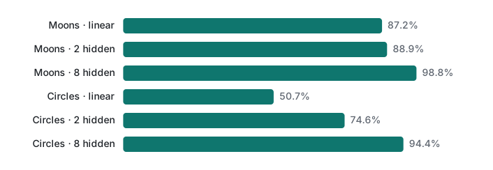
On two moons the linear model is not bad: 87.2%. The moons overlap only at their tips, and a tilted line gets most points right. Two hidden units add almost nothing (88.9%), and four units jump to 99.0%. Beyond that, extra units bought no accuracy and cost linear time: 16 units took 4.43 s per run against 1.45 s for 4.
On circles the linear model scores 50.7%, which is chance. No line separates a ring from the disc inside it. Two hidden units give 74.6% (two lines can cut off a band, not a ring). Eight reach 94.4%, and the rings overlap enough under noise 0.15 that 100% is not reachable. Note the spread for 4 units: 87.7% to 94.8% across five seeds. Report several seeds or you will report luck.
Training time in pure Python
Every number above is CPython executing nested for loops over lists. One SGD update of the 2-8-1 network (forward, backward, step) costs about 13 µs: 2.42 s for 600 samples × 300 epochs = 180,000 updates. The 2-16-1 network takes about 25 µs per update (4.43 s), so the cost grows roughly linearly with hidden size, as the loop structure predicts. Logistic regression, with three parameters inlined into one loop, takes 0.7 µs per update (0.13 s).
That is fine for learning and for a few thousand points with a handful of features. It is not fine for images or text embeddings. A 784-input, 128-hidden layer needs about 100,000 multiply-adds per sample in the forward pass alone, against 24 here. Our 2-8-1 net has 33 parameters and costs 13 µs per update, about 0.4 µs per parameter. At that rate one update of a 100,000-weight layer would take on the order of 40 ms per sample. That gap is the reason the frameworks exist.
What changes with ReLU, softmax and frameworks
We did not install or run any of these here. This is what would change, in words:
- ReLU (
max(0, z)) replaces tanh in most hidden layers today. Its derivative is just 1 or 0, so it is cheaper and does not saturate for positive inputs, which matters in deep stacks where tanh derivatives multiply into tiny numbers. Its own failure mode is the "dead" unit that outputs 0 for every input and therefore never receives a gradient. It is a cousin of the collapse we measured. - Softmax with cross-entropy generalises our sigmoid output to K classes. The useful fact carries over unchanged: the output error is still
y − t, with t now a one-hot vector. Ourdz2 = y - tline becomes a vector subtraction. - Initialisation schemes (Xavier/Glorot for tanh, He for ReLU) scale the initial range by the layer's fan-in. Our ±0.5 vs ±1.0 vs ±2.0 table shows why someone bothered to name them: on XOR, the range alone moved success from 0% to 54% with the same two hidden units.
- Frameworks (PyTorch, TensorFlow, JAX) replace
backwardwith automatic differentiation. You writeforwardand callloss.backward(). They also run the loops as vectorised C/CUDA kernels and offer optimisers like Adam that adapt the step per parameter. Gradient checking does not disappear. Frameworks expose it for custom operations, because a hand-written derivative is still the most common place for a silent bug.
Linear model or hidden layer: a decision table
| Situation | Choose | Evidence from this article |
|---|---|---|
| Classes separable by a line (AND, OR) | Perceptron / logistic regression | AND in 6 epochs, OR in 4 |
| Nearly separable, overlap only at edges | Start linear and measure the gap | Moons: 87.2% linear vs 98.8% with 8 hidden units |
| Class depends on an interaction (XOR, "A or B but not both") | Hidden layer, or a hand-made feature such as x1·x2 | Perceptron loops forever; the 2-H-1 net solves it |
| One class surrounds the other (rings, radius-based) | Hidden layer, or a feature such as x1² + x2² | Circles: 50.7% linear vs 94.4% with 8 hidden units |
| You need to explain each weight | Linear | A weight per feature has a direct meaning |
| Training must be cheap in pure Python | Linear | 0.13 s vs 2.42 s per run on 600 points |
| Small network gets stuck often | More hidden units, wider init, or sigmoid/other activation | tanh ±1.0: 41% → 97% from 2 to 8 units |
If a single engineered feature makes the data linear (x1·x2 for XOR, the radius for circles), that is often the better answer: it is faster, explainable and never gets stuck. The hidden layer earns its cost when you do not know which feature to build.
Honest limits
- XOR is four points. "Success rate" here measures how training behaves, not how well a network generalises. The success rates depend on our choices: learning rate 0.5, plain SGD, zero-initialised biases, a 0.1 tolerance and a 5,000-epoch limit. Change any of them and the numbers move.
- The collapse explanation is our reading of the measured weights (1e-49 everywhere, outputs at 0.5). We did not prove it. We also did not establish why the sigmoid hidden layer avoids it. We only observed that none of our 600 sigmoid runs collapsed; all 60 sigmoid failures (2 hidden units) were local minima.
- One dataset seed. Moons and circles were generated once (seed 7), with five training seeds each. A different noise level changes which hidden size is "enough".
- No regularisation, no validation split, no early stopping. With 16 units on 600 points, overfitting was not visible here, but on real data it would be.
- Measured on Python 3.9.6 only. The code uses only
math,randomandtime, with nothing deprecated, so it should run unchanged on 3.12+. Timings will differ there, since newer CPython is faster on this kind of loop. - ReLU, softmax and frameworks are described, not measured. Nothing was installed for this article.
The next lecture leaves neural networks and goes back to text: ranking our own posts with TF-IDF and BM25, where there are no labels to learn from at all.
FAQ
How often does a small neural network get stuck on XOR?
With a tanh hidden layer, weights drawn from ±1.0 and SGD at learning rate 0.5, 2 hidden units solved XOR in 41 of 100 seeds, 4 units in 73 and 8 units in 97. Most failures were not local minima: the weights shrank to about 1e-49 and the network answered 0.5 for every input.
How do I check that my backpropagation is correct?
Compare each analytic gradient with a central difference (L(w+eps) − L(w−eps)) / 2eps. With eps = 1e-4 our 17-parameter network matched to 1.6e-9 at most; a deliberately broken backward pass (missing tanh derivative) showed a difference of 0.33.
When is a linear model enough?
When the classes are separated by a line, or nearly so. On two moons logistic regression reached 87.2% test accuracy against 98.8% for an 8-unit network. On concentric circles it scored 50.7%, a coin flip, while the network reached 94.4%.